
Rで決定木分析(rpartによるCARTとrangerによるランダムフォレスト)
概要
準備
決定木(decision tree)分析をする際、まず目的変数の種類とアルゴリズムを決定する。
アルゴリズム
- CART
- CHAID
- ID3 / C4.5 / C5.0
目的変数の型
目的変数の型によって扱いが変わる
- 質的変数(2値変数):分類木→目的変数が0/1, T/Fの場合は
as.factor()でfactor型にデータ変換しておく - 量的変数:回帰木
- survivalオブジェクト
- (生起を表す2カラム)
CARTはすべて対応、C4.5/C5.0は質的変数のみ
ここではCARTアルゴリズムでツリーモデルを生成するrpartと、ランダムフォレストrangerを中心に説明する。
データセットと前処理
Default of Credit Card Clients Dataset データセットの主な留意点
- 30000行25変数
- 最初の列が識別子(
ID)→除外 - 3列目
SEX, 4列目EDUCATION, 5列目MARRIAGEがカテゴリ変数→factorに変換 - 最終列
default.payment.next.monthが目的変数で0/1の値をとる。 - それ以外は数値型変数なので型変換の必要なし
以上の処理をしたデータのうち80%を学習データ、20%をテストデータとして分割する。
require(data.table)

data.dt <- fread("UCI_Credit_Card.csv")
data.dt[,ID:=NULL]
data.dt[,SEX:=as.factor(SEX)]
data.dt[,EDUCATION:=as.factor(EDUCATION)]
data.dt[,MARRIAGE:=as.factor(MARRIAGE)]

nr <- nrow(data.dt)
train <- sample(nr, nr*0.8)
train.dt <- data.dt[train] # 学習データ
test.dt <- data.dt[-train] # 検証データ
1回限りの決定木
実行
require(rpart)
train.dt |>
  mutate(
    default.payment.next.month = as.factor(default.payment.next.month == 1)
  ) |>
  rpart(
    formula = default.payment.next.month ~ .,
    data = _,
    method = 'class',
    parms = list(split='information'),
    control = rpart.control(minsplit = 10, cp= .001)
  ) -> rpart_model
- dplyrのパイプ内でdata.tableを渡す場合、
mutateの結果はtibble/data.frameになる。rpartはdata.frameをそのまま受け付ける - 投入するデータテーブルの変数を絞っておくと変数指定が楽
- プロットしたときのラベルをわかりやすく変換しておくといい
- 分類木の場合は目的変数をfactor型に変換しておく
- 重要なパラメータ
method(通常は目的変数の型によって自動で最適なものが選択される)- ‘class’で分類木(目的変数がfactor型)
- ‘poisson’で生起(目的変数が2カラムの生起データ)
- ’exp’で生存(目的変数がsurvivalオブジェクト)
- ‘anova’で回帰木(目的変数が上記のいずれでもない)
parms:method = 'class'の場合、以下の指標に基づいて分割。method = 'anova'の場合は指定しないparms = list(split='gini')でジニ係数を使う(デフォルト)parms = list(split='information')でエントロピーを使う
rpart.controlminsplitは1ノードのサイズの下限cpは小さいほど細かく分岐する。あとで粗くできるので最初は細かく分けておくといい
見る
summary(rpart_model)
出力
Call:
rpart(formula = default.payment.next.month ~ ., data = ., method = "class",
    parms = list(split = "information"), control = rpart.control(minsplit = 10,
        cp = 0.001))
  n= 24000

           CP nsplit rel error    xerror       xstd
1 0.184880240      0 1.0000000 1.0000000 0.01206064
2 0.002245509      1 0.8151198 0.8151198 0.01117344
3 0.002151946      4 0.8074476 0.8197979 0.01119832
4 0.001060379      7 0.8003368 0.8197979 0.01119832
5 0.001000000     10 0.7971557 0.8203593 0.01120130

Variable importance
   PAY_0    PAY_2    PAY_5    PAY_4    PAY_3    PAY_6 PAY_AMT3
      66       18        4        3        3        3        1

Node number 1: 24000 observations,    complexity param=0.1848802
  predicted class=FALSE  expected loss=0.2226667  P(node) =1
    class counts: 18656  5344
   probabilities: 0.777 0.223
  left son=2 (21510 obs) right son=3 (2490 obs)
  Primary splits:
      PAY_0 < 1.5      to the left,  improve=1478.1780, (0 missing)
      PAY_2 < 1.5      to the left,  improve=1168.7680, (0 missing)
      PAY_3 < 1.5      to the left,  improve= 869.5735, (0 missing)
      PAY_4 < 0.5      to the left,  improve= 758.7756, (0 missing)
      PAY_5 < 1        to the left,  improve= 689.8890, (0 missing)
  Surrogate splits:
      PAY_4 < 2.5      to the left,  agree=0.900, adj=0.037, (0 split)
      PAY_5 < 2.5      to the left,  agree=0.900, adj=0.035, (0 split)
      PAY_3 < 2.5      to the left,  agree=0.899, adj=0.029, (0 split)
      PAY_6 < 2.5      to the left,  agree=0.899, adj=0.028, (0 split)
      PAY_2 < 3.5      to the left,  agree=0.898, adj=0.018, (0 split)

    :
変数の重要度を確認
rpart_model$variable.importance
出力
       PAY_0        PAY_2        PAY_5        PAY_4        PAY_3
1478.1783401  395.1016287   80.8746934   75.6083311   70.7895234
       PAY_6     PAY_AMT3    BILL_AMT1     PAY_AMT4    BILL_AMT2
  62.3976688   11.4724819   11.0370003   10.9009460    9.7894688
    PAY_AMT5    EDUCATION    BILL_AMT3    BILL_AMT5    BILL_AMT4
   8.6928210    7.0296988    5.4445876    5.1257181    4.7143508
   BILL_AMT6     PAY_AMT6          AGE     PAY_AMT1
   4.5410328    3.5949029    0.5542719    0.2771359
チューニング(cpを調整)
cpはツリーモデルの複雑さを表すパラメータ。値が小さいものほどモデルが細かくなる。
cpを見る
printcp(rpart_model)
plotcp(rpart_model)
出力
Classification tree:
rpart(formula = default.payment.next.month ~ ., data = ., method = "class",
    parms = list(split = "information"), control = rpart.control(minsplit = 10,
        cp = 0.001))

Variables actually used in tree construction:
 [1] BILL_AMT1 EDUCATION PAY_0     PAY_2     PAY_3     PAY_5     PAY_6
 [8] PAY_AMT3  PAY_AMT4  PAY_AMT5

Root node error: 5344/24000 = 0.22267

n= 24000

         CP nsplit rel error  xerror     xstd
1 0.1848802      0   1.00000 1.00000 0.012061
2 0.0022455      1   0.81512 0.81512 0.011173
3 0.0021519      4   0.80745 0.81980 0.011198
4 0.0010604      7   0.80034 0.81980 0.011198
5 0.0010000     10   0.79716 0.82036 0.011201
cpを調整(cpの小さいツリーモデルからcpの大きいツリーモデルへ)
rpart_model_new <- prune(rpart_model, cp=0.0022)
プロット(2通りのライブラリで)
ビルトインのplot
par(xpd = TRUE)
plot(rpart_model_new, compress = TRUE)
text(rpart_model_new, use.n = TRUE)
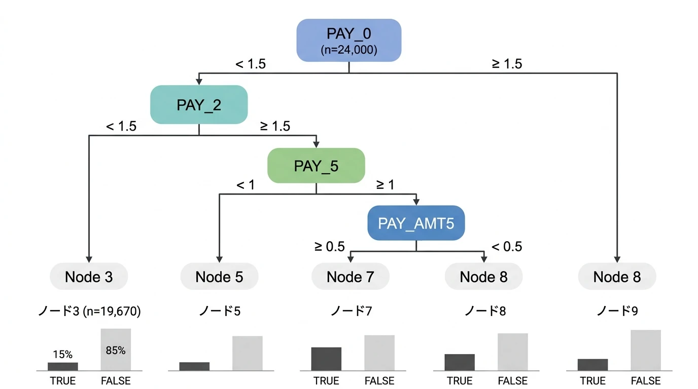
(決定木のプロット例)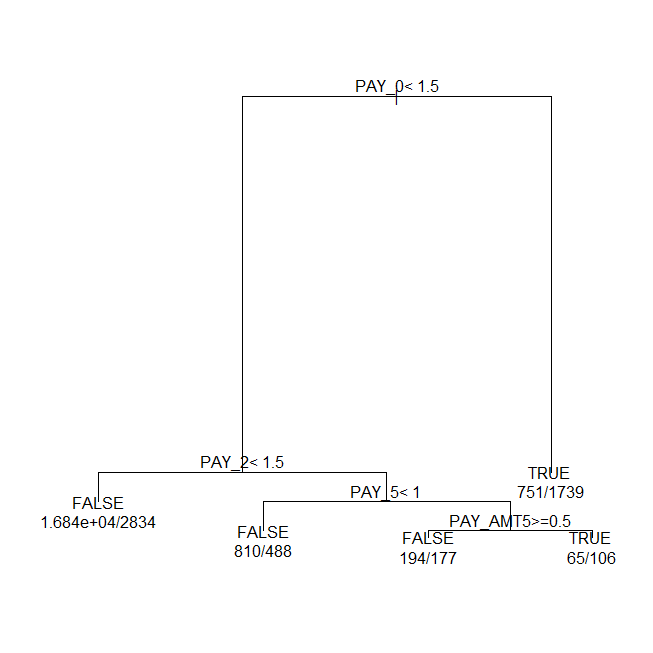
ライブラリ{rpart.plot}
require(rpart.plot)
rpart.plot(rpart_model_new)
(決定木のプロット例)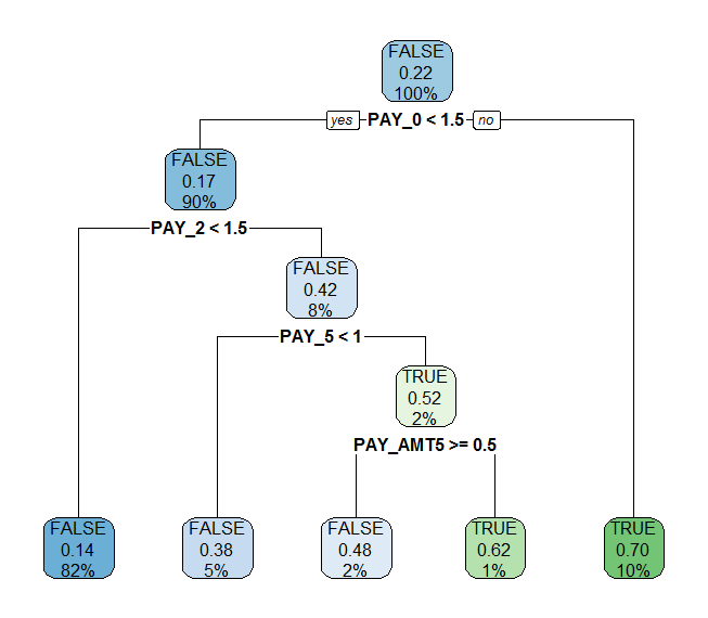
ライブラリ{partykit}
require(partykit)
plot(as.party(rpart_model_new))
plot(as.party(rpart_model_new), gp = gpar(fontsize = 9))
(決定木のプロット例)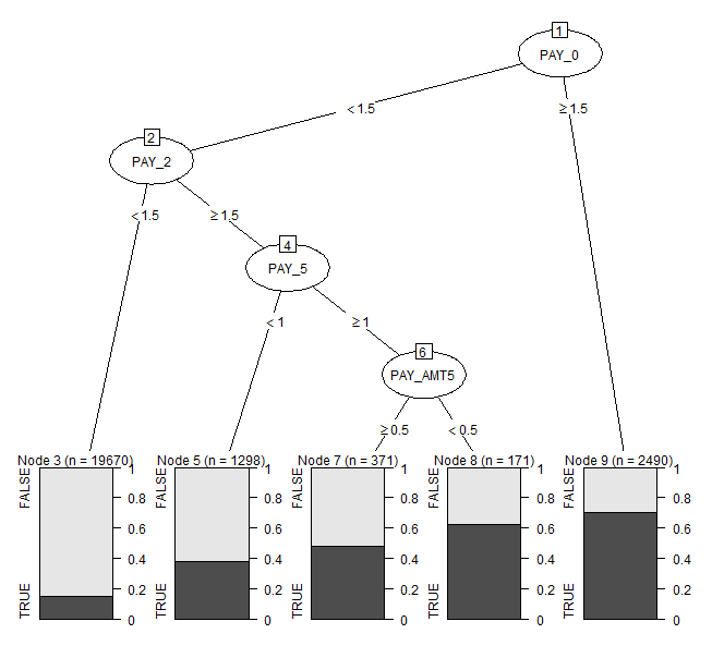
分類されたノードを元データに紐づける
train.dt[, node := rpart_model_new$where]
予測
各クラスに所属する確率を予測する
predict(rpart_model_new, test.dt)
ランダムフォレスト(random forest)
rangerパッケージが便利。
以下の目的変数ごとのツリーモデルをサポートしている。
- 質的変数(2値変数):分類木→目的変数が0/1, T/Fの場合は
as.factor()でfactor型に変換しておく - 量的変数:回帰木
- survivalオブジェクト
実行(モデルの構築)
require(ranger)
require(ROCR)

# モデルの構築
ranger_model <- ranger(
  formula = as.factor(default.payment.next.month) ~ ., # default.payment.next.monthが目的変数になる
  data = train.dt,
  num.trees = 1000,
  mtry = 5,
  write.forest = TRUE,
  importance = 'permutation',
  probability = TRUE
)
パラメータ
ランダムフォレストのハイパーパラメータは
num.trees: 試す決定木の数mtry: モデルに採用する変数の数
mtryをグリッドサーチするならtidymodelsのtune_grid()を使う(後述)。
その他の主なパラメータ
min.node.sizeでノードサイズの下限を指定できるimportanceを指定すると変数の重要度を返す(デフォルトは"none"で重要度は計算されない)"impurity": 不純度ベースの重要度(分類ではジニ係数、回帰では分散減少)- 利点: 計算が高速
- 注意: 相関変数や多カテゴリ変数が過大評価されるバイアスあり
"permutation": 置換ベースの重要度(変数をシャッフルした際の性能劣化)- 利点: 統計的に信頼性が高く、解釈が直感的
- 欠点: 計算時間が長い
- 推奨: 信頼性を重視して
"permutation"を使用。大規模データで計算時間が問題になる場合のみ"impurity"を検討
- 目的変数が質的変数の時、
probability = TRUEで確率を返す。デフォルトのFALSEではT/Fの応答(ただしfactor)を返す。確率は2列の行列で、logical型の目的変数をfactor型にしてranger()をかけている場合、2列目がTRUEとなる(FALSE,TRUEの順)
なおデフォルトでは
- 分類木ではGini係数に基づいて、
- 回帰木では分散に基づいて、
- 生存モデルではログランクに基づいて
分割する。
戻り値
戻り値のrangerオブジェクトはリストで、よく使う属性が
predictionsが予測結果variable.importanceが変数の重要度
なお結果のprediction.errorは
- 分類木では誤分類の割合
- 回帰木では平均二乗誤差(MSE)
- 生存モデルではc-index
が使われる。
予測
predict()関数を使う。新しいデータセットを指定する引数の名前がdata(newdataではない!)
ranger_pred <- predict(ranger_model, data=test.dt)
実行結果が予測結果値そのものではなく、予測結果値を含むリスト。予測結果値は
ranger_pred$predictions
で取り出す。
2値分類時は形式が特殊になる。
ranger()の実行時にprobability = TRUEを指定している場合は1列目がFALSEの確率、2列目がTRUEの確率となる行列
→TRUEとなる確率を取り出すには
ranger_pred <- predict(ranger_model, data=test.dt)$predictions[,2]
probability = FALSEを指定している場合はTRUE/FALSEの結果になる
ranger_pred <- predict(ranger_model, data=test.dt)$predictions
モデルの評価
partial dependence plot
partial dependence plot(部分従属プロット)を描くにはedarfパッケージを使う。ranger以外にもrandomForest, RandomForest, rfsrcのランダムフォレストオブジェクトに対応している。
require(edarf)
pd <- partial_dependence(ranger_model, vars = c('BILL_AMT1', 'PAY_0'), data = as.data.frame(train.dt))
plot_pd(pd)
partial_dependence()の引数dataはdata.tableではダメで、data.frameでなければならない
このパッケージedarfはランダムフォレストの診断に便利。
edarfの解説
精度
{ROCR}パッケージでAUCやROC曲線をプロットできる
ranger_predが結果(レスポンス)の場合、confusion matrix(混同行列)
# 予測結果のレスポンスのベクトルを取り出す
ranger_pred <- predict(ranger_model, data=test.dt)$predictions
# confusion matrix
table(ranger_pred, test.dt[,default.payment.next.month])
ranger_predが確率の場合、AUCを計算する
# 予測結果の確率のベクトルを取り出す
ranger_pred <- predict(ranger_model, data=test.dt)$predictions[,2]
# ROCオブジェクトを生成
rocr_pred <- prediction(ranger_pred, test.dt[,default.payment.next.month])
# ROCオブジェクトからAUCを取り出す
performance(rocr_pred, 'auc')@y.values
ROC曲線
performance(rocr_pred, "tpr", "fpr") |> plot()
{tidymodels}のtune_grid()でハイパーパラメータをグリッドサーチ
caretは新規開発が停止しており、tidymodelsが後継として推奨される。
require(tidymodels)

# 前処理: 目的変数をfactor型に。factorのラベルが整数値だとNGのためmake.namesで変換
train_df <- train.dt |>
  mutate(default.payment.next.month = as.factor(default.payment.next.month)) |>
  mutate(across(where(is.factor), make.names)) |>
  as.data.frame()

# モデル spec(mtryをチューニング)
rf_spec <- rand_forest(mtry = tune(), min_n = 1, trees = 1000) |>
  set_engine("ranger", importance = "permutation") |>
  set_mode("classification")

# ワークフロー
rf_wf <- workflow() |>
  add_formula(default.payment.next.month ~ .) |>
  add_model(rf_spec)

# 交差検証(5分割)
set.seed(123)
cv_folds <- vfold_cv(train_df, v = 5, strata = default.payment.next.month)

# グリッドサーチ
rf_res <- rf_wf |>
  tune_grid(
    resamples = cv_folds,
    grid = expand.grid(mtry = 3:10),
    metrics = metric_set(roc_auc),
    control = control_grid(allow_par = TRUE)
  )

# 最良パラメータ
select_best(rf_res, metric = "roc_auc")
- NAを含む行は
vfold_cvの前にdrop_na()などで除外するか、recipeで処理する metric_set(roc_auc)でROC-AUCを評価指標に指定する
出力例
# A tibble: 1 x 2
   mtry .config
  <int> <chr>
     3  Preprocessor1_Model01
参考 - rpart(決定木)をtidymodelsでチューニング
# 目的変数はfactor型で、ラベルが整数値や「TRUE」「FALSE」だとNGのためmake.namesで変換
train_df_rpart <- train.dt |>
  mutate(default.payment.next.month = as.factor(default.payment.next.month)) |>
  mutate(across(where(is.factor), make.names)) |>
  as.data.frame()

dt_spec <- decision_tree(cost_complexity = tune(), min_n = 10) |>
  set_engine("rpart", parms = list(split = "information")) |>
  set_mode("classification")

dt_wf <- workflow() |>
  add_formula(default.payment.next.month ~ .) |>
  add_model(dt_spec)

set.seed(234)
cv_folds_dt <- vfold_cv(train_df_rpart, v = 10, repeats = 10, strata = default.payment.next.month)

dt_res <- dt_wf |>
  tune_grid(
    resamples = cv_folds_dt,
    grid = 10,
    metrics = metric_set(roc_auc),
    control = control_grid(allow_par = TRUE)
  )

select_best(dt_res, metric = "roc_auc")
cp(cost_complexity)の値を探索することになる。